News

Harish Gudla
CTO at Compular
When you run molecular dynamics simulations of ionic liquid (IL) electrolytes, you eventually have to answer a deceptively simple question: how should I calculate ionic conductivity from my trajectories? Two well-established routes exist: the Nernst–Einstein (NE) formalism and the rigorous Onsager formalism. The choice between them directly affects accuracy and throughput, especially at the high salt concentrations and low temperatures most relevant for battery electrolyte design.
In our recent white paper with Solvionic, we benchmarked simulated density, viscosity, and ionic conductivity against experimental data for three IL electrolyte families (EMIFSI, PYR13FSI, N1113FSI) across a wide matrix of LiFSI concentrations (0-4 M) and temperatures (-10 °C to 60 °C). The conductivity values reported there used the NE formalism. Here we explain why that was the right call, and what happens when you try the alternative.
Two formalisms, one set of trajectories
Both methods start from the same MD trajectories but capture fundamentally different levels of ion-transport physics.
The NE formalism computes conductivity from the self-diffusion coefficients of each ionic species. Because every ion in the simulation box contributes an independent sample at every saved snapshot, the underlying mean-square displacement (MSD) terms converge quickly, even from short production windows (~1.5 ns per replica in our protocol). This convergence advantage holds across all conditions, but it is most impactful precisely where battery electrolytes operate: at high LiFSI concentrations where ion mobility is low and at sub-ambient temperatures where structural relaxation times are long.
The Onsager formalism instead evaluates the full transport coefficient matrix, including off-diagonal cross-correlation terms that capture correlated motion between different ions. This is the formally exact conductivity of the simulated system. However, only one collective-current sample is available per snapshot, so converging those cross terms demands trajectory lengths of 60 to 100 ns or more roughly two orders of magnitude longer than what a high-throughput screening protocol can afford. When the trajectories are too short, the cross terms become non-linear, oscillatory, and noisy, inflating the computed conductivity to unphysical values.
Self and cross MSD decomposition: what the data show
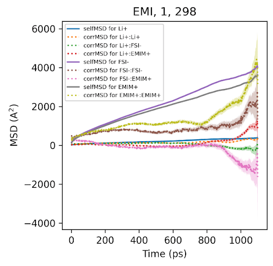
The total conductivity can be decomposed into self terms (individual ion diffusion, corresponding to NE conductivity) and cross terms (correlated motion between different ions). The figure shows both components for EMIFSI with 1 M LiFSI at 298 K.
The self-MSD terms (solid lines) for Li⁺, FSI⁻, and EMI⁺ are linear and well-converged throughout the trajectory window, benefiting from N independent ion samples per snapshot. The cross-correlation terms (dotted lines), by contrast, show increasing non-linearity and noise. The FSI⁻:EMI⁺ pair in particular develops strong curvature and expanding uncertainty bands, signaling poorly sampled anti-correlated motion within the ~1.5 ns window.
This is already visible at 1 M and 298 K. At higher concentrations (3-4 M) and lower temperatures (-10 °C), the problem worsens: ion mobility drops, relaxation times grow, and the cross terms become dominated by rare fluctuations that inflate the Onsager conductivity estimate. The self terms remain stable throughout.
Where this matters most: high-concentration, low-temperature screening
This is also the regime where screening decisions matter most: a formulation that maintains adequate conductivity at 2-3 M LiFSI and -10 °C is far more valuable than one that only works under mild conditions. Across all three IL systems studied in the white paper, the pattern is consistent:
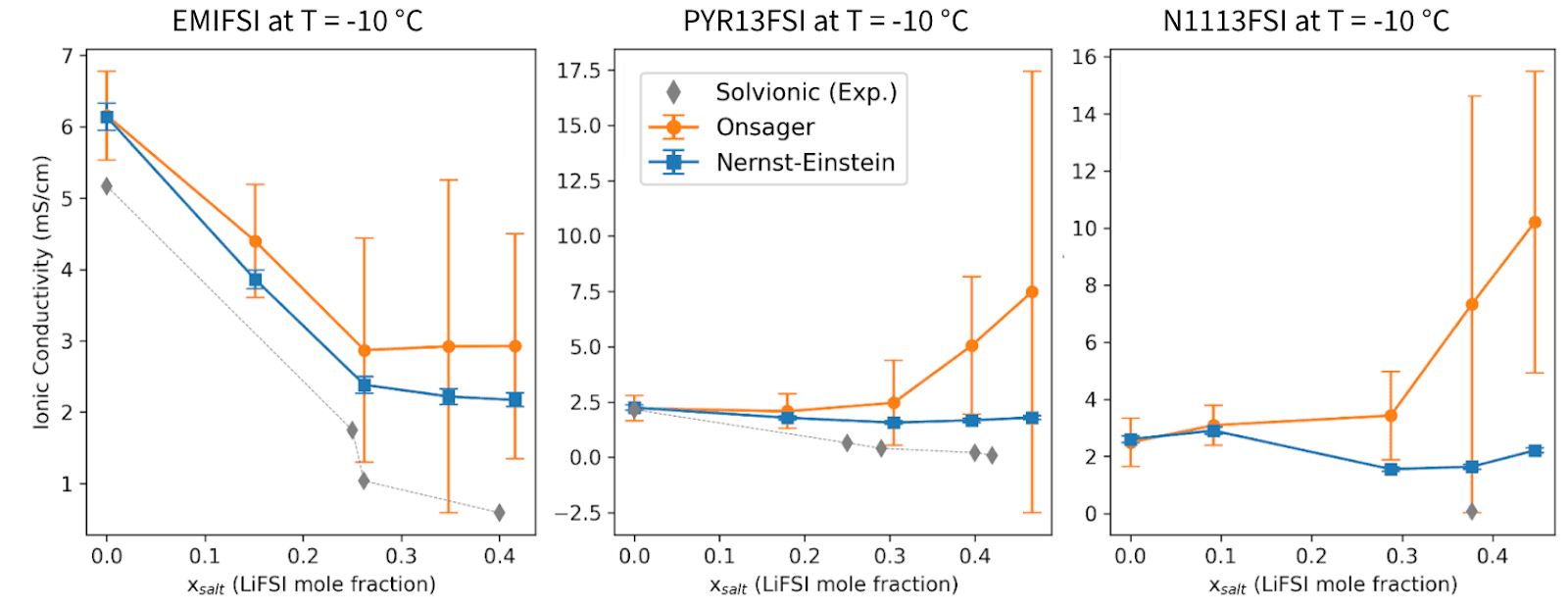
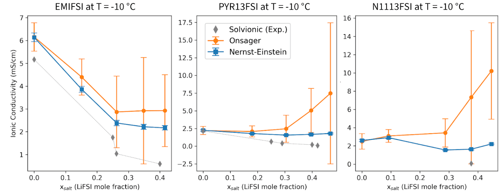
Pure ILs (no LiFSI): NE and Onsager conductivities agree closely because ion-ion correlations are weak and the independent-ion approximation holds well.
Increasing LiFSI concentration: The Onsager conductivity diverges systematically above the NE value with progressively larger error bars. At the most challenging conditions (e.g., N1113FSI at 3-4 M, -10 °C), the Onsager estimate can exceed NE by 3 to 5 times.
Comparison with experiment: Where Solvionic experimental data are available, NE consistently tracks the measured conductivity more closely than the Onsager values, particularly in the 1-3 M LiFSI range and at moderate to high temperatures.
The overestimation by the Onsager method is not a failure of the formalism itself, but a direct consequence of under-converged cross-correlation terms within the accessible trajectory lengths.
The bottom line
The NE formalism is an approximation that neglects ion-ion correlations. With sufficiently long simulations (>100 ns per state point), the Onsager method would be the rigorous approach. However, for screening concentrated, viscous formulations at low operating temperatures, NE is more dependable:
Statistical robustness at challenging conditions: NE converges from short, replica-based protocols and delivers tight error bars under the very conditions (high salt, low temperature) where the Onsager cross terms become most problematic.
Better experimental agreement: NE conductivities match measured values more closely than under-converged Onsager estimates.
Reliable trend prediction across the design space: Both formalisms capture the key ion-transport physics, but with NE formulations one can reliably rank candidate formulations across a broad composition-temperature matrix.
It is important to note that this conclusion is specific to concentrated IL electrolytes where the cross-correlation terms are large, slow to converge, and dominated by anti-correlated ion motion. However, for other kinds of electrolytes, e.g. carbonate based electrolytes around 1 M salt concentration, positive correlations from ion pairing are important, and here a different approach is needed to accelerate beyond the Onsager approach without losing accuracy. In Compular Lab, this is solved by a modified NE approach on the level of dynamic solvated species rather than molecular species, as described here and here.
By pairing the NE formalism with polarizable force fields (APPLE&P) and replica-based sampling, combined with the context awareness of when to apply it on the molecular or cluster level, Compular Lab delivers conductivity estimates that are both computationally efficient and experimentally consistent across the full range of conditions relevant to next-generation battery electrolyte design.
For the full simulation methodology, systems studied, and detailed property comparisons, see the Compular-Solvionic White Paper (December 2025).